Project Introduction
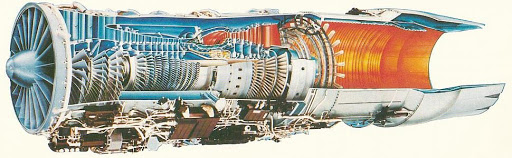
Turbines are often used in many thermodynamic systems. One such system includes the gas turbine engine which is implemented in jet engines. Thermodynamics has shown that an increase in the turbine inlet temperature results in higher efficiency and output, however, this is not possible with many existing systems. This is due to the material properties of the existing technologies. Unfortunately, these systems cannot handle such extreme temperatures without significant deformation and catastrophic breakdown. Some remedies have been created in attempt to reach these higher temperatures without failure occurring. Once such remedy includes creating cooling channels within the part with which cooler fluids can be ran through. The final project of my thermal engineering laboratory involved performing 2D numerical heat transfer analysis of an internally cooled turbine blade.
Problem Statement
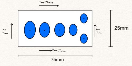
For this project, a singular turbine blade subjected to external heating and internal cooling will be studied. To reduce complexity, the blade geometry is treated as a flat plate 75mm by 25mm in length and width. In addition to geometrical simplifications, the system is treated as having reached steady-state conditions. The material will be inconel with a thermal conductivity of 11.7 W/(mK). Lastly, the cooling channels are treated as energy generation sinks in six distinct locations. Each sink can be represented by an elliptic Gaussian distribution function. Using an iterative solver, contour plots of the energy generation and temperature distribution are plotted and analyzed.
Theory
The finite volume method (FVM) was selected as the method for analysis.
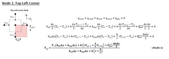
To perform analysis, 9 different nodal equations needed to be created. These include: leading edge (LE) top corner, LE middle, LE bottom corner, middle top, interior, middle bottom, tailing edge (TE) top corner, TE middle, and TE bottom corner. Three example derivations are shown below. The remaining derivations can be found in the PDF of the final report attached at the top.


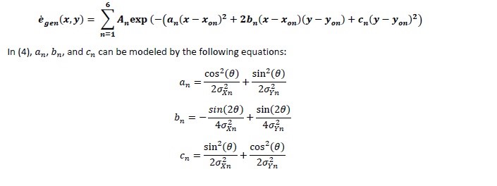
The elliptic Gaussian distribution function describing the heat sinks is shown below.
Analysis
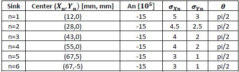
MATLAB code was written to perform the analysis. Different grid sizes of 75×75, 100×100, and 200×200 were used to show how solutions vary based on node count. The following table provides the energy sink distribution parameters used.
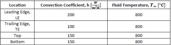
The convective boundary conditions can be found below.
Results
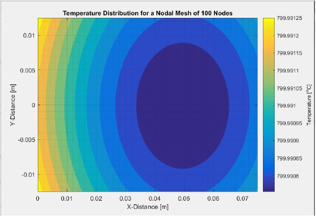
The following image depicts the temperature of the turbine blade without energy generation. As expected, the blade nearly approaches the 800°C almost uniformly.
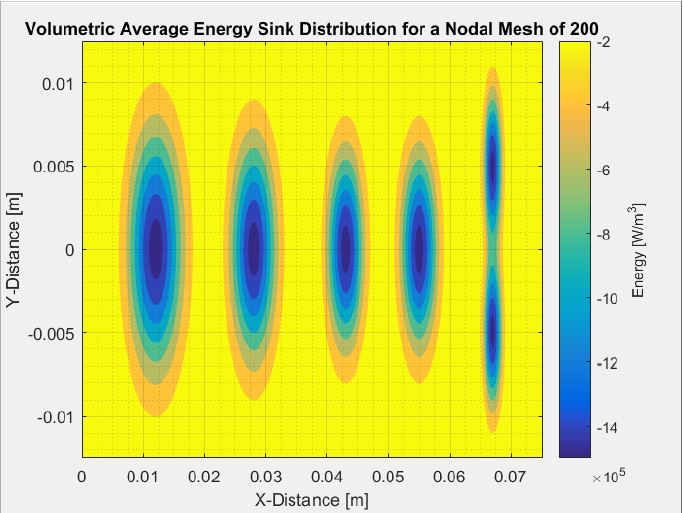
The following contour represents the volumetric average energy sink distribution. The volumetric average was taken to produce a more accurate solution. If the average is not taken, the energy generation will only be evaluated at a single node rather than the entire finite volume. This is accomplished by breaking each finite volume into a small domain and applying a 10×10 grid to it. Energy generation is then evaluated at each internal point within the given node and averaged. For more information, please view the report.
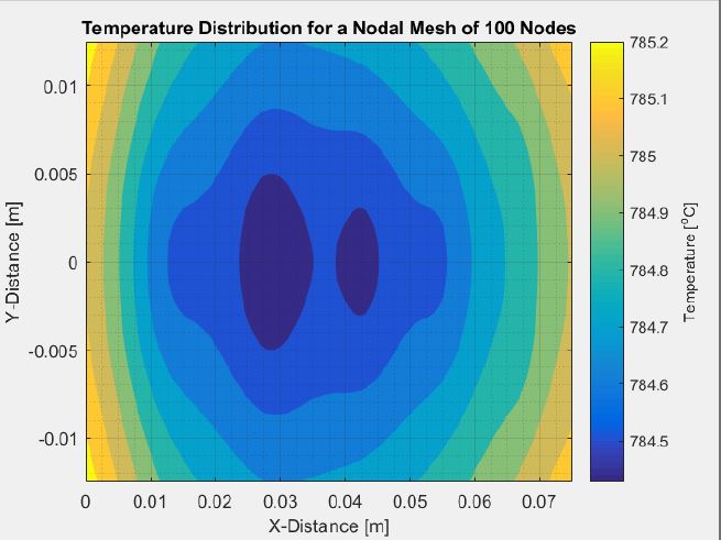
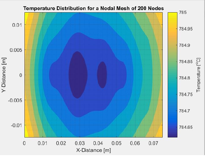
The final contours for all mesh cases can be seen below. The plots display substantially different contours than without energy generation. Note how there is approximately a 15°C drop in temperature when cooling is introduced. Also note how the variation in mesh size influences contour plots and energy conservation.

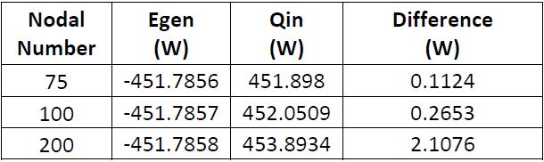
Lastly, the first law of thermodynamics is applied to each scenario to evaluate energy conservation, the results of which are shown below. In each case, energy is not fully conserved. This is an inherent problem introduced in numeric simulations caused by round-off error and convergence criterion. Because the values are relatively low, the solution is deemed viable.